Singularity-free Human Kinematics and Dynamics
Human motion optimization is a crucial task, typically used to clean noisy motion capture data or to ensure physical plausibility. However, human motion is defined as a time sequence of body joint rotations, and performing optimization on rotations is not straightforward. In this article, I will discuss the singularity problem associated with discontinuous rotation representations and introduce a singularity-free approach for modeling human kinematics and dynamics. I have applied this approach to enhance my PIP and PNP work, resulting in a consistent improvement in the accuracy of captured human motion (see results).
Let's begin with a toy example
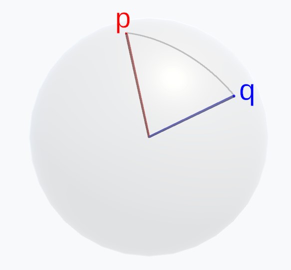
To intuitively illustrate how the singularity of different rotation representations affects the rotation optimization problem, let's begin with a simple example. Consider two 3D unit vectors, \(\boldsymbol p\) and \(\boldsymbol q\). Our goal is to estimate a 3D rotation matrix \(\boldsymbol R\) that rotates \(\boldsymbol p\) to \(\boldsymbol q\). This problem can be formulated as follows: \[\min_{\boldsymbol R} \|\boldsymbol R \boldsymbol p - \boldsymbol q\|^2.\] Although we can easily find the solution to this simple problem, our goal is to solve it through iterative optimization. By plotting the endpoint of the rotated vector at each optimization step, we can visualize the optimization trajectory. Ideally, we want the optimization to be as efficient as possible, i.e., to follow the shortest path that rotates \(\boldsymbol p\) to \(\boldsymbol q\). This shortest path corresponds to the minimal arc between the two points on the unit sphere:
Now, we examine how different rotation representations behave during optimization. We begin with the axis-angle rotation representation, which uses a minimal 3 degrees of freedom (DoF) to encode a 3D rotation: specifically, a unit 3D vector \(\hat{\boldsymbol a}\) for the rotation axis and a scalar \(\theta\) for the angle. We denote the axis-angle representation by \(\boldsymbol \theta = \hat{\boldsymbol a} \theta\), and the corresponding rotation matrix is given by \(\boldsymbol R = \mathrm R\{\boldsymbol \theta\}\). Using this representation, our objective becomes: \[\min_{\boldsymbol \theta} \|\mathrm R\{\boldsymbol \theta\}\boldsymbol p - \boldsymbol q\|^2.\] This is a non-linear least squares problem, which can be solved using the gradient descent method or, more efficiently, the Gauss-Newton algorithm. Defining the residual as \(\boldsymbol e(\boldsymbol \theta) = \mathrm R\{\boldsymbol \theta\}\boldsymbol p - \boldsymbol q\), we can compute the Jacobian \(\boldsymbol J = \frac{\partial \boldsymbol e(\boldsymbol \theta)}{\partial \boldsymbol \theta} = -\mathrm R\{\boldsymbol \theta\}[\boldsymbol p]_\times \boldsymbol J_r\), where \([\cdot]_\times\) maps a 3D vector to the skew-symmetric matrix for the cross product and \(\boldsymbol J_r = \frac{\sin\theta}{\theta}\boldsymbol I + (1 - \frac{\sin\theta}{\theta})\hat{\boldsymbol a}\hat{\boldsymbol a}^T - \frac{1 - \cos\theta}{\theta}[\hat{\boldsymbol a}]_\times\). The derivation is provided below. Note that understanding the derivation requires some additional background in the mathematics of rotations. Skipping this part will not hinder the understanding of the main content of the article. I have condensed parts that are not essential for the overall understanding and made them available for further reading.
Here, we derive the Jacobian of the residual. Using the exponential map \(\mathrm R\{\boldsymbol \theta\} = e^{[\boldsymbol \theta]_\times}\), we have: \[\begin{align} \frac{\partial \boldsymbol e(\boldsymbol \theta)}{\partial \boldsymbol \theta} &= \frac{\partial \mathrm R\{\boldsymbol \theta\}\boldsymbol p}{\partial \boldsymbol \theta} \\ &= \lim_{\delta \boldsymbol \theta \rightarrow 0}\frac{e^{[\boldsymbol \theta + \delta \boldsymbol \theta]_\times} \boldsymbol p - e^{[\boldsymbol \theta]_\times}\boldsymbol p}{\delta \boldsymbol \theta}\\ &= \lim_{\delta \boldsymbol \theta \rightarrow 0}\frac{e^{[\boldsymbol \theta]_\times} e^{[\boldsymbol J_r\delta \boldsymbol \theta]_\times} \boldsymbol p - e^{[\boldsymbol \theta]_\times}\boldsymbol p}{\delta \boldsymbol \theta}\\ &= \lim_{\delta \boldsymbol \theta \rightarrow 0}\frac{e^{[\boldsymbol \theta]_\times} (\boldsymbol I + [\boldsymbol J_r\delta \boldsymbol \theta]_\times) \boldsymbol p - e^{[\boldsymbol \theta]_\times}\boldsymbol p}{\delta \boldsymbol \theta}\\ &= \lim_{\delta \boldsymbol \theta \rightarrow 0}\frac{e^{[\boldsymbol \theta]_\times} [\boldsymbol J_r\delta \boldsymbol \theta]_\times \boldsymbol p}{\delta \boldsymbol \theta}\\ &= \lim_{\delta \boldsymbol \theta \rightarrow 0}\frac{-e^{[\boldsymbol \theta]_\times} [\boldsymbol p]_\times \boldsymbol J_r\delta \boldsymbol \theta}{\delta \boldsymbol \theta}\\ &= -\mathrm R\{\boldsymbol \theta\}[\boldsymbol p]_\times \boldsymbol J_r \end{align}\]
Given \(\nabla_{\boldsymbol \theta}\|\boldsymbol e\|^2=2\boldsymbol e^T\boldsymbol J\), we can write the update equation at each iteration for the gradient descent method (note that we transpose the gradient to convert it into a column vector and omit the constant term): \[\boldsymbol \theta \leftarrow \boldsymbol \theta - \lambda \boldsymbol J^T \boldsymbol e,\] where \(\lambda\) is the step size. For the Gauss-Newton algorithm, the update equation is: \[\boldsymbol \theta \leftarrow \boldsymbol \theta - \alpha \boldsymbol J^\dagger \boldsymbol e,\] where \(\alpha\) controls the step length and \(\cdot^\dagger\) denotes the pseudoinverse. For readers unfamiliar with the Gauss-Newton algorithm, I have provided a straightforward explanation here.
In the Gaussian-Newton algorithm, we begin by assigning an initial value to the optimizable variable, such as setting \(\boldsymbol \theta = \boldsymbol 0\). During each optimization step, the goal is to compute an increment \(\delta \boldsymbol \theta\) such that the residual becomes zero after updating the variable: \(\boldsymbol e(\boldsymbol \theta + \delta \boldsymbol \theta) = \boldsymbol 0\). To achieve this, we linearize the residual at \(\boldsymbol \theta\) as: \[\boldsymbol e(\boldsymbol \theta + \delta \boldsymbol \theta) = \boldsymbol e(\boldsymbol \theta) + \frac{\partial \boldsymbol e}{\partial \boldsymbol \theta}\delta \boldsymbol \theta = \boldsymbol e(\boldsymbol \theta) + \boldsymbol J \delta \boldsymbol \theta = \boldsymbol 0.\] From this, the increment can be computed as the least squares solution by \(\delta \boldsymbol \theta = -\boldsymbol J^\dagger \boldsymbol e\). In practice, we employ a fraction \(\alpha\) of the increment in the update to avoid divergence.
Let's now visualize the optimization trajectory of the axis-angle representation. The initial value of \(\boldsymbol p\) is set to \((1,0,0)^T\), and \(\boldsymbol q\) is randomized ten times after each optimization stage converges. The step size is set to \(0.2\), and the iterations run at 60Hz for visualization. The optimal trajectory (shortest path) for each stage is depicted in gray, while the optimization trajectory is shown in red.
It is evident from the video that optimizing the axis-angle representation does not follow an optimal trajectory. The performance significantly deteriorates as the magnitude of \(\boldsymbol \theta\) increase. This is clearly reflected in the video: the optimization proceeds quickly and effectively when approaching early targets (where \(|\boldsymbol \theta|\) is small), but slows down considerably and deviates from the optimal trajectory as \(|\boldsymbol \theta|\) becomes larger. To mitigate this issue during optimization, a deeper understanding of the singularity in the axis-angle representation is necessary. I provide a deeper analysis below for further reading.
To explain why the optimization performance deteriorates as the magnitude of \(\boldsymbol \theta\) increase, we need to find out the singularity of the axis-angle representation. Given a 3D rotation represented in the axis-angle form \(\boldsymbol \theta\), we analyze the "effort" required to rotate it slightly in an arbitrarily chosen direction. To do this, we first randomly sample a unit 3D vector \(\hat{\boldsymbol \phi}\). Then, we rotate \(\boldsymbol \theta\) around \(\hat{\boldsymbol \phi}\) by a very small angle \(\delta \phi\). Finally, we analyze how much \(\boldsymbol \theta\) changes due to this perturbation: \[\delta \boldsymbol \theta = \log(e^{[\boldsymbol \theta ]_\times}e^{[\hat{\boldsymbol \phi}\delta\phi]_\times})^\vee - \log(e^{[\boldsymbol \theta]_\times})^\vee.\] Using Baker–Campbell–Hausdorff formula and assuming \(\delta\phi\) is small, we have \(\delta \boldsymbol \theta = \boldsymbol J_r^{-1} \hat{\boldsymbol \phi}\delta \phi\) (note \(\boldsymbol J_r\) has also appeared before and let's assume it is invertible). Rearranging the equation, we have: \[\hat{\boldsymbol \phi} = \boldsymbol J_r \frac{\delta \boldsymbol \theta}{\delta \phi}.\] Given that \(\hat{\boldsymbol \phi}\) is a unit vector, we have: \[1 = \hat{\boldsymbol \phi}^T\hat{\boldsymbol \phi} = \frac{1}{\delta\phi^2}\delta \boldsymbol \theta^T \boldsymbol J_r^T\boldsymbol J_r \delta\boldsymbol\theta.\] We denote \(\boldsymbol A = (\boldsymbol J_r^T\boldsymbol J_r)^{-1}\) and \(\boldsymbol x = \frac{\delta \boldsymbol \theta}{\delta \phi}\). It's easy to demonstrate \(\boldsymbol A\) is both symmetric and positive definite. The equation above becomes:\[1=\boldsymbol x^T\boldsymbol A^{-1}\boldsymbol x,\] which defines a 3D ellipsoid of \(\boldsymbol x\) values. We care about the longest axis among the three principal axes of the ellipsoid, as it represents the most "difficult" direction to perturb the rotation. Its length, \(|\boldsymbol x| = \frac{|\delta\boldsymbol\theta|}{\delta\phi}\), indicates how much the angle \(\delta\phi\) needs to be scaled to achieve the perturbation using the axis-angle representation. Actually, the longest principal axis of an ellipsoid corresponds to the eigenvector associated with the largest eigenvalue of \(\boldsymbol A\). The half-length of this axis is equal to the square root of the largest eigenvalue: \[\max\frac{|\delta\boldsymbol\theta|}{\delta\phi} = \sqrt{\rho(A)} = \|\boldsymbol J_r^{-1}\|_2,\] where \(\rho(\boldsymbol A)\) represents the largest eigenvalue of \(\boldsymbol A\), and \(\sqrt{\rho(\boldsymbol A)}\) is exactly the spectral norm of \(\boldsymbol J_r^{-1}\). Let's denote \(s=\|\boldsymbol J_r^{-1}(\boldsymbol \theta)\|_2\), which serves as a good indicator of the singularity of the axis-angle representation \(\boldsymbol \theta\). It is easy to demonstrate that \(s\) is invariant to the direction of \(\boldsymbol \theta\) and depends only on its magnitude, i.e., \(s=s(\theta)\). I have derived the analytical formula of \(s\) by computing the spectral norm: \[s(\theta)=\max\frac{|\delta\boldsymbol\theta|}{\delta\phi}=\left|\frac{\theta}{2}\csc\frac{\theta}{2}\right|.\] Below, I plot \(s(\theta)\) as a function of \(\theta\) in \([-2\pi,2\pi]\):
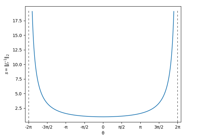
Let’s interpret what the plot of \(s(\theta)\) means: given a 3D rotation in axis-angle representation \(\boldsymbol \theta\), if we want to apply a small perturbation to it, we actually need a maximum effort proportional to \(s(\theta)\) to adjust the axis-angle representation. The optimal value of \(s\) is 1 (at \(\boldsymbol \theta = \boldsymbol 0\)), which indicates that the effort required to change the representation matches the effort required for the actual rotation.
From the plot, it becomes evident that the singularity of the axis-angle representation occurs at a magnitude of \(\pm 2\pi\), where \(s\) approaches infinity. This implies that as \(\boldsymbol \theta\) nears this singularity, it becomes increasingly difficult (essentially impossible) to rotate in certain directions by operating the axis-angle representation. Examining the eigenvectors reveals that these directions are all orthogonal to the direction of \(\boldsymbol \theta\). This explains the poor performance during optimization with the axis-angle representation. Readers can recheck the \(s\) values in the video for further understanding: when \(s\) approaches \(2\pi\) (during Target 4 and 5), the gradient descent method becomes extremely slow, while the Gauss-Newton method becomes highly unstable due to the singularity.
To alleviate this issue, a practical approach is to always normalize the axis-angle representation within the range \([-\pi, \pi]\), effectively avoiding such singularities (though this introduces discontinuities). Below, I visualize the optimization trajectory of the axis-angle representation with such normalization. The optimization becomes significantly faster and more stable. However, it can still be observed that the optimization trajectory does not strictly follow the optimal one.
Similar to the axis-angle representation, all 3-dimensional representations of rotation suffer from singularity issues. For example, the Euler angle representation is prone to the Gimbal lock problem. If one chooses to use these 3D representations, it is essential to carefully account for their singularities to prevent optimization from stalling or deviating significantly.
TBC...